Calculus: The Mathematics of Change

By Nowsherwan Khan (Team Research)

Newton’s Invention

We have all heard of how Newton discovered gravity after an apple fell from a tree. What we all haven’t heard is that Newton was working on the motion of the Earth and the Moon. He wanted to know more about their motion and the physical laws that govern them. One day, he saw an apple falling from a tree. He looked at the apple and then looked at the sky and asked the question:

“If the apple falls, does the Moon also fall?’’

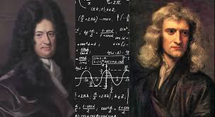
Newton started to develop the mathematics for motion of a falling Moon. He realized that the 17^th century was not enough to describe the motion of the moon. He started working on the mathematics, and invented a new branch of mathematics called ‘’Calculus”. (Calculus was independently discovered by Gottfried Wilhelm Leibniz as well).

The remarkable progress that has been made in science and technology during the last century is due in large part to the development of mathematics. That branch of mathematics known as “integral and differential calculus” serves as a natural and powerful tool for attacking a variety of problems that arise in physics, astronomy, engineering, chemistry, geology, biology, and other fields including, rather recently, some of the social sciences.

Now, what is calculus?

Calculus is the mathematics of motion and change. Where there is motion or growth, where variable forces are at work producing acceleration, calculus is the right mathematics to apply. This was true in the beginning of the subject, and it is true today. The needs in the 17^th century were mainly mechanical in nature. Differential calculus dealt with the problem of calculating rates of change. It enabled people to define the slopes of curves. To calculate velocities and accelerations of moving bodies, to find firing angles that would give cannons their greatest range, and to predict the times when planets would be closest together or farthest apart. Integral calculus dealt with the problem of determining a function from information about its rate of change. It enabled people to calculate the future location of a body from its present position – and knowledge of the forces acting on it – to find the areas of irregular regions in the plane, to measure the lengths of curves, and to find the volumes and masses of arbitrary solids.

Today, calculus and its extensions in mathematical analysis are far reaching indeed, and physicists, mathematicians, and astronomers – who first invented the subject, would surely be amazed and delighted, as the amount of problems that can be solved with calculus is enormous.

With what speed should a rocket be fired upward so that it never returns to earth? What is the radius of the smallest circular disk that can cover every isosceles triangle of a given perimeter L? What volume of material is removed from a solid sphere of radius 2r if a hole of radius r is drilled through the center? If a strain of bacteria grows at a rate proportional to the amount present, and if the population doubles in one hour, by how much will it increase at the end of two hours? If a ten-pound force stretches an elastic spring one inch, how much work is required to stretch the spring one foot?

These examples, chosen from various fields, illustrate some of the technical questions that can be answered by more or less routine applications of calculus.

Mainly in calculus we want to find two things:

1. the rate of change (differential calculus)
2. the area under a curve (integral calculus)

Some of the important concepts of calculus are explained here briefly:

Limits

Limits are a part of differential calculus. Limits deal with limiting values. Suppose you have a function f(x)= x², and someone asks you what the value of lim x tends to 2, f(x), be. What does it mean?

If you plot the graph of y=x², you will get an upward parabola. Now you are asked what is the limiting y=x², when x is tending to 2?

If you substitute y=2², you get 4. So as x, the input variable is tending to 2, your output is tending to 4.

What is important to note here? The term x tending to 2 means that x is getting very very closer to 2, e.g. 2.0000000001 or 1.99999999.

Your limit will exist only if your left-hand limit and right-hand limit are equal.

In the above example, left hand approaching to 2 means that from the left of the number line – i.e. 1.9999999, and right hand approaching to 2 means from the right of number line – i.e. 2.000000001.

Now, you must be wondering, “what are the uses of limits?”

Using limits, we can calculate the limiting value of a function, or its behavior if the input is approaching a specific value. This is very important to know the behavior of functions, because if you know how a function is behaving at some values of input, you can tell a lot about the outputs and its future behavior. Notice that in the above example, y=x², you would get 4 if you put 2, not just if you approach 2…. So what’s the difference? The answer is the limiting value and the actual value at that point are not always the same.

Example

(x² − 1)(x − 1)

Let’s work it out for x = 1:

(1²− 1)(1 − 1) = (1 − 1)(1 − 1) = 0/0

Now 0/0 is a difficulty! We don’t really know the value of 0/0 (it is “indeterminate”), so we need another way of answering this.

So, instead of trying to work it out for x=1, let’s try approaching it closer and closer:

x	(x2 − 1)(x − 1)
0.5	1.50000
0.9	1.90000
0.99	1.99000
0.999	1.99900
0.9999	1.99990
0.99999	1.99999
….	….

We see that as x gets close to 1, then (x²−1)(x−1) gets close to 2.

We are now faced with an interesting situation:

• When x=1 we don’t know the answer (it is indeterminate)
• But we can see that it is going to be 2

We want to give the answer “2” but can’t, so instead mathematicians say exactly what is going on by using the special word “limits”:

The limit of (x²−1)(x−1) as x approaches 1 is 2.

And it is written in symbols as:

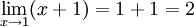
limx→1x²−1x−1 = 2

So it is a special way of saying, “ignoring what happens when we get there, but as we get closer and closer the answer gets closer and closer to 2“

How to solve it? Well, we can use factorization.

Example

By factoring (x²−1) into (x−1)(x+1) we get:

We can just substitute x=1 to get the limit:

We now know the behavior of this function if the input variable is approaching to 1.

You can read part-II of this blog here